Basic relations

We are going to postulate the following things about the Kalman filter

The Kalman filter algorithm directly emerges from Bayes' Thereom (we are going to show this below)
The Linear Kalman filter is the best estimator in case we are dealing only with Gaussian probability density functions
The Linear Kalman filter algorithm consists of two parts - prediction and update/correction - which can be executed continuously one after each other, while carrying the probability density function at any given epoch.

For any multivariate Gaussian state of dimension , we can express its Gaussian probability density function as

$\begin{equation} \label{eq:eq-Gaussian} p(\boldsymbol{x})=\det((2\pi)^n\boldsymbol{\Sigma})^{-\frac{1}{2}}\cdot \exp\left(-\frac{1}{2}(\boldsymbol{x}-\boldsymbol{\mu})^T\boldsymbol{\Sigma}^{-1}(\boldsymbol{x}-\boldsymbol{\mu})\right) \end{equation}$

The basic idea of the Kalman filter is that both, prediction and update are represented by linear function/transformations between the state-space respectively the observation space.

$\begin{equation} \label{eq:eq-predictation_and_observation_model} \begin{aligned} \boldsymbol{x}_t&=\boldsymbol{\Phi}_t\boldsymbol{x}_{t-1}+\boldsymbol{B}_t\boldsymbol{u}_t+\boldsymbol{\varepsilon}_t\\ \boldsymbol{z}_t&=\boldsymbol{H}_t\boldsymbol{x}_t+\boldsymbol{\upsilon}_t \end{aligned} \end{equation}$

The following table summarizes the meaning of these variables.

Variable	Meaning
$\boldsymbol{\Phi}_t$	$(n\times n)$ state transition matrix, which describes the linear relation between the state at time and .
$\boldsymbol{B}_t$	(linear) control-input model which is applied to the control vector $\boldsymbol{u}_t$ (note: in many cases ) $\boldsymbol{u}_t$ is zero, in particular when we deal with an error-state Kalman filter
$\boldsymbol{H}_t$	observation model, which linearly maps the state space into the observation space
$\boldsymbol{\varepsilon}_t$	process noise, which is assumed to be drawn from a zero mean multivariate normal distribution, with covariance $\boldsymbol{Q}_t$ so that $\boldsymbol{\varepsilon}_t \sim \mathcal{N}( \boldsymbol{0},\boldsymbol{Q}_t )$
$\boldsymbol{\upsilon}_t$	observation noise, which is assumed to be zero mean Gaussian white noise with covariance $\boldsymbol{R}_t$ so that $\boldsymbol{\upsilon}_t \sim \mathcal{N}( \boldsymbol{0},\boldsymbol{R}_t )$

Considering now that we have a linear prediction model described above, one can compute the Gaussian probability density function after predication as

$\begin{equation} \label{eq:eq-prediction} p(\boldsymbol{x}_t\, |\,\boldsymbol{u}_t,\boldsymbol{x}_{t-1})=\det((2\pi)^n\boldsymbol{Q}_t)^{-\frac{1}{2}}\cdot \exp\left(-\frac{1}{2}(\boldsymbol{x}_t-\boldsymbol{\Phi}_t\boldsymbol{x}_{t-1}-\boldsymbol{B}_t\boldsymbol{u}_t)^T\boldsymbol{Q}^{-1}_t(\boldsymbol{x}_t-\boldsymbol{\Phi}_t\boldsymbol{x}_{t-1}-\boldsymbol{B}_t\boldsymbol{u}_t)\right). \end{equation}$

In a similar way, one can derive the Gaussian probability density function after after making noisy observations as

$\begin{equation} \label{eq:eq-measurement} p(\boldsymbol{z}_t\, |\,\boldsymbol{x}_t)=\det((2\pi)^m\boldsymbol{R}_t)^{-\frac{1}{2}}\cdot \exp\left(-\frac{1}{2}(\boldsymbol{z}_t-\boldsymbol{H}_t\boldsymbol{x}_t)^T\boldsymbol{R}^{-1}_t(\boldsymbol{z}_t-\boldsymbol{H}_t\boldsymbol{x}_t)\right) \end{equation}$

.

Bayes' Theorem

Assumption (not proven here): Prediction and update of states with underlying Gaussian distributions lead to Gaussian distributions again. Thus, one can make use of Bayes' Theorem which states that prediction can be understood as convolution of the prior probability density function (PDF), here called "belief" $bel(\boldsymbol{x}_t)$ with the PDF of the prediction. This means, prediction can be understood as

$\begin{equation} \label{eq:eq-Bayes-prediction} bel^-(\boldsymbol{x}_t)=\int {p(\boldsymbol{x}_t\, |\,\boldsymbol{u}_t,\boldsymbol{x}_{t-1})}\cdot {bel(\boldsymbol{x}_{t-1})}\cdot d\boldsymbol{x}_{t-1} \end{equation}$

where superscript ${\,}^{-}$ indicates that we obtain a predicted belief from this equation. Moreover, we know from Bayes' Theorem that observation of a state is equal to multiplication of the PDF of the (predicted belief) with PDF of the observation. This means

$\begin{equation} \label{eq:eq-Bayes-update} bel(\boldsymbol{x}_t)^+=\eta\cdot p(\boldsymbol{z}_t\, |\,\boldsymbol{x}_t)\cdot bel^-(\boldsymbol{x}_t) \end{equation}$

where superscript ${\,}^{+}$ indicates that we obtain a new belief after making an observation which depends on the state. The factor $\eta$ makes sure that the obtained Gaussian fulfills the normalization criteria, i.e. its hyper-volume is equal to .

Using Bayes' Theorem for Prediction

Putting the PDF for prediction into Bayes' Theorem we obtain

$\begin{equation} \label{eq:eq-Bayes-prediction01} bel^-(\boldsymbol{x}_t) =\eta\int \exp\left(-\frac{1}{2}(\boldsymbol{x}_t-\boldsymbol{\Phi}_t\boldsymbol{x}_{t-1}-\boldsymbol{B}_t\boldsymbol{u}_t)^T\boldsymbol{Q}^{-1}_t(\boldsymbol{x}_t-\boldsymbol{\Phi}_t\boldsymbol{x}_{t-1}-\boldsymbol{B}_t\boldsymbol{u}_t)\right) \exp\left(-\frac{1}{2}(\boldsymbol{x}_{t-1}-\boldsymbol{\mu}_{t-1})^T\boldsymbol{\Sigma}^{-1}_{t-1}(\boldsymbol{x}_{t-1}-\boldsymbol{\mu}_{t-1})\right)\cdot d\boldsymbol{x}_{t-1} \end{equation}$

where $\boldsymbol{\mu}_{t-1}$ represents the expectation value of the belief before prediction. This can be formally written as

$\begin{equation} \label{eq:eq-Bayes-prediction02} bel^-(\boldsymbol{x}_t)=\eta\int \exp(-L_t)\cdot d\boldsymbol{x}_{t-1} \end{equation}$

where

$\begin{equation} \label{eq:eq-Bayes-prediction03} L_t=\frac{1}{2}(\boldsymbol{x}_t-\boldsymbol{\Phi}_t\boldsymbol{x}_{t-1}-\boldsymbol{B}_t\boldsymbol{u}_t)^T\boldsymbol{Q}^{-1}_t(\boldsymbol{x}_t-\boldsymbol{\Phi}_t\boldsymbol{x}_{t-1}-\boldsymbol{B}_t\boldsymbol{u}_t) +\frac{1}{2}(\boldsymbol{x}_{t-1}-\boldsymbol{\mu}_{t-1})^T\boldsymbol{\Sigma}^{-1}_{t-1}(\boldsymbol{x}_{t-1}-\boldsymbol{\mu}_{t-1}). \end{equation}$

The basic idea is now to split so that it contains two terms, from which only one depends on $\boldsymbol{x}_t$ , i.e.

$\begin{equation} \label{eq:eq-Bayes-prediction04} L_t=L_t(\boldsymbol{x}_{t-1},\boldsymbol{x}_t)+L_t(\boldsymbol{x}_t). \end{equation}$

Thus we obtain

$\begin{equation} \label{eq:eq-Bayes-prediction05} bel^-(\boldsymbol{x}_t)=\eta\int \exp\left \{-L_t(\boldsymbol{x}_{t-1},\boldsymbol{x}_t)-L_t(\boldsymbol{x}_t)\right\}\cdot d\boldsymbol{x}_{t-1} \end{equation}$

which can be simplified to

$\begin{equation} \label{eq:eq-Bayes-prediction06} bel^-(\boldsymbol{x}_t)=\eta\cdot \exp\left \{-L_t(\boldsymbol{x}_t)\right\}\int \exp\left \{-L_t(\boldsymbol{x}_{t-1},\boldsymbol{x}_t)\right\}\cdot d\boldsymbol{x}_{t-1} \end{equation}$

since the term $L_t(\boldsymbol{x}_t)$ can be extracted from the integral as it does not depend on $\boldsymbol{x}_{t-1}$ . Moreover, as we know that the outcome from this function must be a Gaussian again, we can write this as

$\begin{equation} \label{eq:eq-Bayes-prediction07} bel^-(\boldsymbol{x}_t)=\eta'\cdot \exp\left \{-L_t(\boldsymbol{x}_t)\right\} \end{equation}$

The Gaussian probability density function reaches its highest value for its the expectation value. Thus, if we differentiate the exponent in the Gaussian PDF and set the result equal to zero we find its expectation value. Thus, we find

$\begin{equation} \label{eq:eq-Bayes-prediction08} \frac{\partial L_t}{\partial \boldsymbol{x}_{t-1}} = \boldsymbol{0} =-\boldsymbol{\Phi}^T_t\boldsymbol{Q}^{-1}_t(\boldsymbol{x}_t-\boldsymbol{\Phi}_t\boldsymbol{x}_{t-1}-\boldsymbol{B}_t\boldsymbol{u}_t)+\boldsymbol{\Sigma}^{-1}_{t-1}(\boldsymbol{x}_{t-1}-\boldsymbol{\mu}_{t-1}) \end{equation}$

which yields

$\begin{equation} \label{eq:eq-Bayes-prediction09} \boldsymbol{\Phi}^T_t\boldsymbol{Q}^{-1}_t(\boldsymbol{x}_t-\boldsymbol{\Phi}_t\boldsymbol{x}_{t-1}-\boldsymbol{B}_t\boldsymbol{u}_t)=\boldsymbol{\Sigma}^{-1}_{t-1}(\boldsymbol{x}_{t-1}-\boldsymbol{\mu}_{t-1})\\[2mm] \end{equation}$

This can be further re-arranged to

$\begin{eqnarray} \label{eq:eq-Bayes-prediction10} \boldsymbol{\Phi}^T_t\boldsymbol{Q}^{-1}_t(\boldsymbol{x}_t-\boldsymbol{B}_t\boldsymbol{u}_t)-\boldsymbol{\Phi}^T_t\boldsymbol{Q}^{-1}_t\boldsymbol{\Phi}_t\boldsymbol{x}_{t-1}=\boldsymbol{\Sigma}^{-1}_{t-1}\boldsymbol{x}_{t-1}-\boldsymbol{\Sigma}^{-1}_{t-1}\boldsymbol{\mu}_{t-1}\\ \boldsymbol{\Phi}^T_t\boldsymbol{Q}^{-1}_t\boldsymbol{\Phi}_t\boldsymbol{x}_{t-1}+\boldsymbol{\Sigma}^{-1}_{t-1}\boldsymbol{x}_{t-1}=\boldsymbol{\Phi}^T_t\boldsymbol{Q}^{-1}_t(\boldsymbol{x}_t-\boldsymbol{B}_t\boldsymbol{u}_t)+\boldsymbol{\Sigma}^{-1}_{t-1}\boldsymbol{\mu}_{t-1}\\ (\boldsymbol{\Phi}^T_t\boldsymbol{Q}^{-1}_t\boldsymbol{\Phi}_t+\boldsymbol{\Sigma}^{-1}_{t-1})\boldsymbol{x}_{t-1}=\boldsymbol{\Phi}^T_t\boldsymbol{Q}^{-1}_t(\boldsymbol{x}_t-\boldsymbol{B}_t\boldsymbol{u}_t)+\boldsymbol{\Sigma}^{-1}_{t-1}\boldsymbol{\mu}_{t-1} \end{eqnarray}$

Moreover, we know that double differentiation of the exponent provides us with the information matrix / weight matrix, i.e. the inverse of the covariance matrix. Thus, we obtain

$\begin{equation} \label{eq:eq-Bayes-prediction11} \frac{\partial^2 L_t}{\partial \boldsymbol{x}^2_{t-1}}=\boldsymbol{\Phi}^T_t\boldsymbol{Q}^{-1}_t\boldsymbol{\Phi}^T_t+\boldsymbol{\Sigma}^{-1}_{t-1}=:\boldsymbol{\Psi}^{-1}_t \end{equation}$

which we can use to find an alternative notation for the findings before

$\begin{eqnarray} \label{eq:eq-Bayes-prediction12} \Leftrightarrow\qquad&\boldsymbol{\Psi}^{-1}_t\boldsymbol{x}_{t-1}=\boldsymbol{\Phi}^T_t\boldsymbol{Q}^{-1}_t(\boldsymbol{x}_t-\boldsymbol{B}_t\boldsymbol{u}_t)+\boldsymbol{\Sigma}^{-1}_{t-1}\boldsymbol{\mu}_{t-1}\\ \Leftrightarrow\qquad&\boldsymbol{x}_{t-1}=\boldsymbol{\Psi}_t\left( \boldsymbol{\Phi}^T_t\boldsymbol{Q}^{-1}_t(\boldsymbol{x}_t-\boldsymbol{B}_t\boldsymbol{u}_t)+\boldsymbol{\Sigma}^{-1}_{t-1}\boldsymbol{\mu}_{t-1} \right) \end{eqnarray}$

Therefore we can re-write the exponent as

$\begin{equation} \label{eq:eq-Bayes-prediction13} L_t(\boldsymbol{x}_{t-1},\boldsymbol{x}_t) =\frac{1}{2}\left \{\boldsymbol{x}_{t-1}- \boldsymbol{\Psi}_t\left( \boldsymbol{\Phi}^T_t\boldsymbol{Q}^{-1}_t(\boldsymbol{x}_t-\boldsymbol{B}_t\boldsymbol{u}_t)+\boldsymbol{\Sigma}^{-1}_{t-1}\boldsymbol{\mu}_{t-1} \right) \right\}^T\boldsymbol{\Psi}^{-1}_t \left \{\boldsymbol{x}_{t-1}- \boldsymbol{\Psi}_t\left( \boldsymbol{\Phi}^T_t\boldsymbol{Q}^{-1}_t(\boldsymbol{x}_t-\boldsymbol{B}_t\boldsymbol{u}_t)+\boldsymbol{\Sigma}^{-1}_{t-1}\boldsymbol{\mu}_{t-1} \right) \right\} \end{equation}$

Now we are able to compute the term which only one depends on $\boldsymbol{x}_t$

$\begin{equation} \label{eq:eq-Bayes-prediction14} L_t(\boldsymbol{x}_t)=L_t-L_t(\boldsymbol{x}_{t-1},\boldsymbol{x}_t) =\frac{1}{2}(\boldsymbol{x}_t-\boldsymbol{\Phi}_t\boldsymbol{x}_{t-1}-\boldsymbol{B}_t\boldsymbol{u}_t)^T\boldsymbol{Q}^{-1}_t(\boldsymbol{x}_t-\boldsymbol{\Phi}_t\boldsymbol{x}_{t-1}-\boldsymbol{B}_t\boldsymbol{u}_t) +\frac{1}{2}(\boldsymbol{x}_{t-1}-\boldsymbol{\mu}_{t-1})^T\boldsymbol{\Sigma}^{-1}_{t-1}(\boldsymbol{x}_{t-1}-\boldsymbol{\mu}_{t-1}) -\frac{1}{2}\left \{\boldsymbol{x}_{t-1}- \boldsymbol{\Psi}_t\left( \boldsymbol{\Phi}^T_t\boldsymbol{Q}^{-1}_t(\boldsymbol{x}_t-\boldsymbol{B}_t\boldsymbol{u}_t)+\boldsymbol{\Sigma}^{-1}_{t-1}\boldsymbol{\mu}_{t-1} \right) \right\}^T\boldsymbol{\Psi}^{-1}_t \left \{\boldsymbol{x}_{t-1}- \boldsymbol{\Psi}_t\left( \boldsymbol{\Phi}^T_t\boldsymbol{Q}^{-1}_t(\boldsymbol{x}_t-\boldsymbol{B}_t\boldsymbol{u}_t)+\boldsymbol{\Sigma}^{-1}_{t-1}\boldsymbol{\mu}_{t-1} \right) \right\} \end{equation}$

This leads to

$\begin{equation} \label{eq:eq-Bayes-prediction15} L_t(\boldsymbol{x}_t)=\underline{\underline{\frac{1}{2}\boldsymbol{x}^T_{t-1}\boldsymbol{\Phi}^T_t\boldsymbol{Q}^{-1}_t\boldsymbol{\Phi}_t\boldsymbol{x}_{t-1}}}\underline{-\boldsymbol{x}^T_{t-1}\boldsymbol{\Phi}^T_t\boldsymbol{Q}^{-1}_t(\boldsymbol{x}_t-\boldsymbol{B}_t\boldsymbol{u}_t)} +\frac{1}{2}(\boldsymbol{x}_t-\boldsymbol{B}_t\boldsymbol{u}_t)^T\boldsymbol{Q}^{-1}_t(\boldsymbol{x}_t-\boldsymbol{B}_t\boldsymbol{u}_t) \underline{\underline{+\frac{1}{2}\boldsymbol{x}^T_{t-1}\boldsymbol{\Sigma}^{-1}_{t-1}\boldsymbol{x}_{t-1}}}\underline{-\boldsymbol{x}^T_{t-1}\boldsymbol{\Sigma}^{-1}_{t-1}\boldsymbol{\mu}_{t-1}}+\frac{1}{2}\boldsymbol{\mu}^T_{t-1}\boldsymbol{\Sigma}^{-1}_{t-1}\boldsymbol{\mu}_{t-1} \underline{\underline{-\frac{1}{2}\boldsymbol{x}^T_{t-1}(\boldsymbol{\Phi}^T_t\boldsymbol{Q}^{-1}_t\boldsymbol{\Phi}_t+\boldsymbol{\Sigma}^{-1}_{t-1})\boldsymbol{x}_{t-1}}} \underline{+\boldsymbol{x}^T_{t-1}\left(\boldsymbol{\Phi}^T_t\boldsymbol{Q}^{-1}_t(\boldsymbol{x}_t-\boldsymbol{B}_t\boldsymbol{u}_t)+\boldsymbol{\Sigma}^{-1}_{t-1}\boldsymbol{\mu}_{t-1}\right)} -\frac{1}{2}\left( \boldsymbol{\Phi}^T_t\boldsymbol{Q}^{-1}_t(\boldsymbol{x}_t-\boldsymbol{B}_t\boldsymbol{u}_t)+\boldsymbol{\Sigma}^{-1}_{t-1}\boldsymbol{\mu}_{t-1} \right)^T(\boldsymbol{\Phi}^T_t\boldsymbol{Q}^{-1}_t\boldsymbol{\Phi}_t+\boldsymbol{\Sigma}^{-1}_{t-1})^{-1} \left( \boldsymbol{\Phi}^T_t\boldsymbol{Q}^{-1}_t(\boldsymbol{x}_t-\boldsymbol{B}_t\boldsymbol{u}_t)+\boldsymbol{\Sigma}^{-1}_{t-1}\boldsymbol{\mu}_{t-1} \right) \end{equation}$

which simplifies to

$\begin{equation} \label{eq:eq-Bayes-prediction16} L_t(\boldsymbol{x}_t)=\frac{1}{2}(\boldsymbol{x}_t-\boldsymbol{B}_t\boldsymbol{u}_t)^T\boldsymbol{Q}^{-1}_t(\boldsymbol{x}_t-\boldsymbol{B}_t\boldsymbol{u}_t)+\frac{1}{2}\boldsymbol{\mu}^T_{t-1}\boldsymbol{\Sigma}^{-1}_{t-1}\boldsymbol{\mu}_{t-1}-\frac{1}{2}\left( \boldsymbol{\Phi}^T_t\boldsymbol{Q}^{-1}_t(\boldsymbol{x}_t-\boldsymbol{B}_t\boldsymbol{u}_t)+\boldsymbol{\Sigma}^{-1}_{t-1}\boldsymbol{\mu}_{t-1} \right)^T(\boldsymbol{\Phi}^T_t\boldsymbol{Q}^{-1}_t\boldsymbol{\Phi}_t+\boldsymbol{\Sigma}^{-1}_{t-1})^{-1} \left( \boldsymbol{\Phi}^T_t\boldsymbol{Q}^{-1}_t(\boldsymbol{x}_t-\boldsymbol{B}_t\boldsymbol{u}_t)+\boldsymbol{\Sigma}^{-1}_{t-1}\boldsymbol{\mu}_{t-1} \right) \end{equation}$

Based on this, we can differentiate w.r.t. to $\boldsymbol{x}_t$ in order to obtain the expectation value, i.e.

$\begin{equation} \label{eq:eq-Bayes-prediction17} \frac{\partial L_t(\boldsymbol{x}_t)}{\partial \boldsymbol{x}_t}= \boldsymbol{0} = \boldsymbol{Q}^{-1}_t(\boldsymbol{x}_t-\boldsymbol{B}_t\boldsymbol{u}_t)-\boldsymbol{Q}^{-1}_t\boldsymbol{\Phi}_t(\boldsymbol{\Phi}^T_t\boldsymbol{Q}^{-1}_t\boldsymbol{\Phi}_t+\boldsymbol{\Sigma}^{-1}_{t-1})^{-1} \left( \boldsymbol{\Phi}^T_t\boldsymbol{Q}^{-1}_t(\boldsymbol{x}_t-\boldsymbol{B}_t\boldsymbol{u}_t)+\boldsymbol{\Sigma}^{-1}_{t-1}\boldsymbol{\mu}_{t-1} \right) \end{equation}$

respectively,

$\begin{equation} \label{eq:eq-Bayes-prediction18} \boldsymbol{0}=\left(\boldsymbol{Q}^{-1}_t-\boldsymbol{Q}^{-1}_t\boldsymbol{\Phi}_t(\boldsymbol{\Phi}^T_t\boldsymbol{Q}^{-1}_t\boldsymbol{\Phi}_t+\boldsymbol{\Sigma}^{-1}_{t-1})^{-1} \boldsymbol{\Phi}^T_t\boldsymbol{Q}^{-1}_t\right)(\boldsymbol{x}_t-\boldsymbol{B}_t\boldsymbol{u}_t) \end{equation}$

If we use the matrix lemma

$\begin{equation} \label{eq:eq-Bayes-prediction19} \boldsymbol{Q}^{-1}_t-\boldsymbol{Q}^{-1}_t\boldsymbol{\Phi}_t(\boldsymbol{\Phi}^T_t\boldsymbol{Q}^{-1}_t\boldsymbol{\Phi}_t+\boldsymbol{\Sigma}^{-1}_{t-1})^{-1} \boldsymbol{\Phi}^T_t\boldsymbol{Q}^{-1}_t=(\boldsymbol{Q}_t+\boldsymbol{\Phi}_t\boldsymbol{\Sigma}_{t-1}\boldsymbol{\Phi}^T_t)^{-1}\\[6mm] \end{equation}$

We can further simplify and obtain

$\begin{equation} \label{eq:eq-Bayes-prediction20} \frac{\partial L_t(\boldsymbol{x}_t)}{\partial \boldsymbol{x}_t}=\boldsymbol{0}= (\boldsymbol{Q}_t+\boldsymbol{\Phi}_t\boldsymbol{\Sigma}_{t-1}\boldsymbol{\Phi}^T_t)^{-1}(\boldsymbol{x}_t-\boldsymbol{B}_t\boldsymbol{u}_t) -\boldsymbol{Q}^{-1}_t\boldsymbol{\Phi}_t(\boldsymbol{\Phi}^T_t\boldsymbol{Q}^{-1}_t\boldsymbol{\Phi}_t+\boldsymbol{\Sigma}^{-1}_{t-1})^{-1}\boldsymbol{\Sigma}^{-1}_{t-1}\boldsymbol{\mu}_{t-1} \end{equation}$

which turns out to read as

$\begin{equation} \label{eq:eq-Bayes-prediction21} (\boldsymbol{Q}_t+\boldsymbol{\Phi}_t\boldsymbol{\Sigma}_{t-1}\boldsymbol{\Phi}^T_t)^{-1}(\boldsymbol{x}_t-\boldsymbol{B}_t\boldsymbol{u}_t)=\boldsymbol{Q}^{-1}_t\boldsymbol{\Phi}_t(\boldsymbol{\Phi}^T_t\boldsymbol{Q}^{-1}_t\boldsymbol{\Phi}_t+\boldsymbol{\Sigma}^{-1}_{t-1})^{-1}\boldsymbol{\Sigma}^{-1}_{t-1}\boldsymbol{\mu}_{t-1} \end{equation}$

This can be written also as

$\begin{eqnarray} \label{eq:eq-Bayes-prediction22} \boldsymbol{x}_t&=\boldsymbol{B}_t\boldsymbol{u}_t+\underset{\boldsymbol{\Phi}_t+\boldsymbol{\Phi}_t\boldsymbol{\Sigma}_{t-1}\boldsymbol{\Phi}^T_t\boldsymbol{Q}^{-1}_t\boldsymbol{\Phi}_t}{\underbrace{(\boldsymbol{Q}_t+\boldsymbol{\Phi}_t\boldsymbol{\Sigma}_{t-1}\boldsymbol{\Phi}^T_t)^{-1}\boldsymbol{Q}^{-1}_t\boldsymbol{\Phi}_t}}\cdot \underset{(\boldsymbol{\Sigma}_{t-1}\boldsymbol{\Phi}^T_t\boldsymbol{Q}^{-1}_t\boldsymbol{\Phi}_t+\boldsymbol{I})^{-1}}{\underbrace{(\boldsymbol{\Phi}^T_t\boldsymbol{Q}^{-1}_t\boldsymbol{\Phi}_t+\boldsymbol{\Sigma}^{-1}_{t-1})^{-1}\boldsymbol{\Sigma}^{-1}_{t-1}}}\boldsymbol{\mu}_{t-1}\notag\\ &=\boldsymbol{B}_t\boldsymbol{u}_t+\boldsymbol{\Phi}_t\cdot\underset{=\boldsymbol{I}}{\underbrace{(\boldsymbol{I}+\boldsymbol{\Sigma}_{t-1}\boldsymbol{\Phi}^T_t\boldsymbol{Q}^{-1}_t\boldsymbol{\Phi}_t)(\boldsymbol{\Sigma}_{t-1}\boldsymbol{\Phi}^T_t\boldsymbol{Q}^{-1}_t\boldsymbol{\Phi}_t+\boldsymbol{I})^{-1}}}\cdot\boldsymbol{\mu}_{t-1}\notag\\ &=\boldsymbol{B}_t\boldsymbol{u}_t+\boldsymbol{\Phi}_t\boldsymbol{\mu}_{t-1} \end{eqnarray}$

We also find the covariance after prediction, from the second derivative, i.e.

$\begin{equation} \label{eq:eq-Bayes-prediction23} \frac{\partial^2 L_t(\boldsymbol{x}_t)}{\partial \boldsymbol{x}^2_t}=(\boldsymbol{Q}_t+\boldsymbol{\Phi}_t\boldsymbol{\Sigma}_{t-1}\boldsymbol{\Phi}^T_t)^{-1} \quad \Rightarrow \quad \bar{\boldsymbol{\Sigma}}_t^{-1} = (\boldsymbol{Q}_t+\boldsymbol{\Phi}_t\boldsymbol{\Sigma}_{t-1}\boldsymbol{\Phi}^T_t)^{-1} \end{equation}$

Thus, in summary we could prove that the prediction step in the linear Kalman filter turns out to be rather simple, ie.

$\begin{eqnarray} \label{eq:eq-Bayes-prediction_final} \boldsymbol{\mu}_t^-&=\boldsymbol{\Phi}_t\boldsymbol{\mu}_{t-1}+\boldsymbol{B}_t\boldsymbol{u}_t\\ \boldsymbol{\Sigma}_t^-&=\boldsymbol{\Phi}_t\boldsymbol{\Sigma}_{t-1}\boldsymbol{\Phi}^T_t+\boldsymbol{Q}_t \end{eqnarray}$

where the superscript indicates, that we deal with the predicted state and the covariance, respectively.

Using Bayes' Theorem for Update/Correction

As for the update step (we will call it ''update'' hereafter although one might also see it as ''correction'' step), we start with Bayes' Theorem that tell us the conditional likelihood in case we observe an uncertain state. This can be written as

$\begin{equation} \label{eq:eq-Bayes-update01} bel(\boldsymbol{x}_t)=\boldsymbol{\eta}\cdot\underset{\sim\mathcal{N}(\boldsymbol{z}_t;\boldsymbol{H}_t\boldsymbol{x}_t,\boldsymbol{R}_t)}{\underbrace{p(\boldsymbol{z}_t\, |\,\boldsymbol{x}_t)}}\cdot \underset{\sim\mathcal{N}(\boldsymbol{x}_t;\boldsymbol{\mu}_t^{-},\boldsymbol{\Sigma}_t^{-})}{\underbrace{\overline{bel}(\boldsymbol{x}_t)}} \end{equation}$

where $\boldsymbol{\eta}$ is a factor that normalizes the product on the right side, so that a proper PDF is obtained. Knowing know that everything is Gaussian, including the term on the left side, we can write above's equation as

$\begin{equation} \label{eq:eq-Bayes-update02} bel(\boldsymbol{x}_t)=\boldsymbol{\eta}\cdot exp\{-\boldsymbol{J}_t\} \end{equation}$

where

$\begin{equation} \label{eq:eq-Bayes-update03} \boldsymbol{J}_t=\frac{1}{2}(\boldsymbol{z}_t-\boldsymbol{H}_t\boldsymbol{x}_t)^T\boldsymbol{R}^{-1}_t(\boldsymbol{z}_t-\boldsymbol{H}_t\boldsymbol{x}_t)+\frac{1}{2}(\boldsymbol{x}_t-\boldsymbol{\mu}_t^{-})^T(\boldsymbol{\Sigma}_t^{-})^{-1}(\boldsymbol{x}_t-\boldsymbol{\mu}_t^{-}) \end{equation}$

Like before, we can find the expectation value of this function, by differentiating the term $\boldsymbol{J}_t$ and setting the result equal to zero.This means

$\begin{equation} \label{eq:eq-Bayes-update04} \frac{\partial\boldsymbol{J}_t}{\partial \boldsymbol{x}_t}=\boldsymbol{0} = -\boldsymbol{H}^T_t\boldsymbol{R}^{-1}_t(\boldsymbol{z}_t-\boldsymbol{H}_t\boldsymbol{x}_t)+(\boldsymbol{\Sigma}_t^{-})^{-1}(\boldsymbol{x}_t-\boldsymbol{\mu}_t^{-}) \end{equation}$

which can be rearranged to

$\begin{equation} \label{eq:eq-Bayes-update05} \boldsymbol{H}^T_t\boldsymbol{R}^{-1}_t(\boldsymbol{z}_t-\boldsymbol{H}_t\boldsymbol{\mu}_t^{+})=(\boldsymbol{\Sigma}_t^{-})^{-1}(\boldsymbol{\mu}_t^{+}-\boldsymbol{\mu}_t^{-}) \end{equation}$

The second derivative of $\boldsymbol{J}_t$ provides us the inverse of the covariance matrix, i.e.

$\begin{equation} \label{eq:eq-Bayes-update06} \frac{\partial^2 \boldsymbol{J}_t}{\partial \boldsymbol{x}^2_t}=\boldsymbol{\Sigma}_t^{-1} \boldsymbol{H}^T_t\boldsymbol{R}^{-1}_t\boldsymbol{H}_t+(\boldsymbol{\Sigma}_t^{-})^{-1} \end{equation}$

which can be rewritten as

$\begin{equation} \label{eq:eq-Bayes-update07} \boldsymbol{\Sigma}_t=(\boldsymbol{H}^T_t\boldsymbol{R}^{-1}_t\boldsymbol{H}_t+(\boldsymbol{\Sigma}_t^{-})^{-1})^{-1}\\[2mm] % 3.37 \end{equation}$

The equation that hold the expectation value can be re-written to

$\begin{eqnarray} \label{eq:eq-Bayes-update08} &\boldsymbol{H}^T_t\boldsymbol{R}^{-1}_t(\boldsymbol{z}_t-\boldsymbol{H}_t\boldsymbol{\mu}_t^{+})\\ &=\boldsymbol{H}^T_t\boldsymbol{R}^{-1}_t(\boldsymbol{z}_t-\boldsymbol{H}_t\boldsymbol{\mu}_t^{+}+\boldsymbol{H}_t\boldsymbol{\mu}_t^{-}-\boldsymbol{H}_t\boldsymbol{\mu}_t^{-})\\ &=\boldsymbol{H}^T_t\boldsymbol{R}^{-1}_t(\boldsymbol{z}_t-\boldsymbol{H}_t\boldsymbol{\mu}_t^{-})-\boldsymbol{H}^T_t\boldsymbol{R}^{-1}_t\boldsymbol{H}_t(\boldsymbol{\mu}_t^{+}-\boldsymbol{\mu}_t^{-}) \end{eqnarray}$

which in turn allows us to identify

$\begin{equation} \label{eq:eq-Bayes-update09} \boldsymbol{H}^T_t\boldsymbol{R}^{-1}_t(\boldsymbol{z}_t-\boldsymbol{H}_t\boldsymbol{\mu}_t^{-})=\underset{=\boldsymbol{\Sigma}^{-1}_t}{\underbrace{(\boldsymbol{H}^T_t\boldsymbol{R}^{-1}_t\boldsymbol{H}_t+(\boldsymbol{\Sigma}_t^{-})^{-1})}}(\boldsymbol{\mu}_t^{+}-\boldsymbol{\mu}_t^{-}) \end{equation}$

Thus, we can write

$\begin{equation} \label{eq:eq-Bayes-update10} \boldsymbol{\Sigma}_t\boldsymbol{H}^T_t\boldsymbol{R}^{-1}_t(\boldsymbol{z}_t-\boldsymbol{H}_t\boldsymbol{\mu}_t^{-})=\boldsymbol{\mu}_t-\boldsymbol{\mu}_t^{-} \end{equation}$

, or by using the so-called Kalman gain

$\begin{equation} \label{eq:eq-Bayes-update11} \boldsymbol{K}_t=\boldsymbol{\Sigma}_t\boldsymbol{H}^T_t\boldsymbol{R}^{-1}_t \end{equation}$

we obtain a very simple rule how the update has to be computed

$\begin{equation} \label{eq:eq-Bayes-update12} \boldsymbol{\mu}_t^{+}=\boldsymbol{\mu}_t^{-}+\boldsymbol{K}_t(\boldsymbol{z}_t-\boldsymbol{H}_t\boldsymbol{\mu}_t^{-}) %3. \end{equation}$

However, we might want a more straightforward expression for the Kalman gain, that contains only the predicted covariance and not the one after making observations. Thus, we do a series of mathematical tricks and obtain

$\begin{eqnarray} \label{eq:eq-Bayes-update13} \boldsymbol{K}_t&=\boldsymbol{\Sigma}_t\boldsymbol{H}^T_t\boldsymbol{R}^{-1}_t\\ &=\boldsymbol{\Sigma}_t\boldsymbol{H}^T_t\boldsymbol{R}^{-1}_t\underset{=\boldsymbol{I}}{\underbrace{(\boldsymbol{H}_t\boldsymbol{\Sigma}_t^{-}\boldsymbol{H}^T_t+\boldsymbol{R}_t)(\boldsymbol{H}_t\boldsymbol{\Sigma}_t^{-}\boldsymbol{H}^T_t+\boldsymbol{R}_t)^{-1}}}\\ &=\boldsymbol{\Sigma}_t(\boldsymbol{H}^T_t\boldsymbol{R}^{-1}_t\boldsymbol{H}_t\boldsymbol{\Sigma}_t^{-}\boldsymbol{H}^T_t+\boldsymbol{H}^T_t\underset{=\boldsymbol{I}}{\underbrace{\boldsymbol{R}^{-1}_t\boldsymbol{R}_t}})(\boldsymbol{H}_t\boldsymbol{\Sigma}_t^{-}\boldsymbol{H}^T_t+\boldsymbol{R}_t)^{-1}\\ &=\boldsymbol{\Sigma}_t(\boldsymbol{H}^T_t\boldsymbol{R}^{-1}_t\boldsymbol{H}_t\boldsymbol{\Sigma}_t^{-}\boldsymbol{H}^T_t+\boldsymbol{H}^T_t)(\boldsymbol{H}_t\boldsymbol{\Sigma}_t^{-}\boldsymbol{H}^T_t+\boldsymbol{R}_t)^{-1}\\ &=\boldsymbol{\Sigma}_t(\boldsymbol{H}^T_t\boldsymbol{R}^{-1}_t\boldsymbol{H}_t\boldsymbol{\Sigma}_t^{-}\boldsymbol{H}^T_t+\underset{=\boldsymbol{I}}{\underbrace{(\boldsymbol{\Sigma}_t^{-})^{-1}\boldsymbol{\Sigma}_t^{-}}}\boldsymbol{H}^T_t)(\boldsymbol{H}_t\boldsymbol{\Sigma}_t^{-}\boldsymbol{H}^T_t+\boldsymbol{R}_t)^{-1}\\ &=\boldsymbol{\Sigma}_t\underset{=\boldsymbol{\Sigma}^{-1}_t}{\underbrace{(\boldsymbol{H}^T_t\boldsymbol{R}^{-1}_t\boldsymbol{H}_t+(\boldsymbol{\Sigma}_t^{-})^{-1})}}\boldsymbol{\Sigma}_t^{-}\boldsymbol{H}^T_t(\boldsymbol{H}_t\boldsymbol{\Sigma}_t^{-}\boldsymbol{H}^T_t+\boldsymbol{R}_t)^{-1}\\ &=\underset{=\boldsymbol{I}}{\underbrace{\boldsymbol{\Sigma}_t\boldsymbol{\Sigma}^{-1}_t}}\boldsymbol{\Sigma}_t^{-}\boldsymbol{H}^T_t(\boldsymbol{H}_t\boldsymbol{\Sigma}_t^{-}\boldsymbol{H}^T_t+\boldsymbol{R}_t)^{-1}\\ &=\boldsymbol{\Sigma}_t^{-}\boldsymbol{H}^T_t(\boldsymbol{H}_t\boldsymbol{\Sigma}_t^{-}\boldsymbol{H}^T_t+\boldsymbol{R}_t)^{-1} \end{eqnarray}$

We can also find an easier expression for the updated covariance matrix, if we use a matrix lemma and reformulate

$\begin{equation} \label{eq:eq-Bayes-update14} ((\boldsymbol{\Sigma}_t^{-})^{-1}+\boldsymbol{H}^T_t\boldsymbol{R}^{-1}_t\boldsymbol{H}_t)^{-1}=\boldsymbol{\Sigma}_t^{-}-\boldsymbol{\Sigma}_t^{-}\boldsymbol{H}^T_t(\boldsymbol{R}_t+\boldsymbol{H}_t\boldsymbol{\Sigma}_t^{-}\boldsymbol{H}^T_t)^{-1}\boldsymbol{H}^T_t\boldsymbol{\Sigma}_t^{-} \end{equation}$

With that we obtain

$\begin{eqnarray} \label{eq:eq-Bayes-update15} \boldsymbol{\Sigma}_t&=(\boldsymbol{H}^T_t\boldsymbol{R}^{-1}_t\boldsymbol{H}_t+(\boldsymbol{\Sigma}_t^{-})^{-1})^{-1}\\ &=\boldsymbol{\Sigma}_t^{-}-\boldsymbol{\Sigma}_t^{-}\boldsymbol{H}^T_t(\boldsymbol{R}_t+\boldsymbol{H}_t\boldsymbol{\Sigma}_t^{-}\boldsymbol{H}^T_t)^{-1}\boldsymbol{H}_t\boldsymbol{\Sigma}_t^{-}\\ &=[\boldsymbol{I}-\underset{=\boldsymbol{K}_t}{\underbrace{\boldsymbol{\Sigma}_t^{-}\boldsymbol{H}^T_t(\boldsymbol{R}_t+\boldsymbol{H}_t\boldsymbol{\Sigma}_t^{-}\boldsymbol{H}^T_t)^{-1}}}\boldsymbol{H}_t]\boldsymbol{\Sigma}_t^{-}\\ &=(\boldsymbol{I}-\boldsymbol{K}_t\boldsymbol{H}_t)\boldsymbol{\Sigma}_t^{-} \end{eqnarray}$

Putting everything together we find for the update step the following very simple rules

$\begin{eqnarray} \label{eq:eq-Bayes-update-final} \boldsymbol{K}_t&=\boldsymbol{\Sigma}_t^{-}\boldsymbol{H}^T_t(\boldsymbol{H}_t\boldsymbol{\Sigma}_t^{-}\boldsymbol{H}^T_t+\boldsymbol{R}_t)^{-1}\\ \boldsymbol{\mu}_t^{+}&=\boldsymbol{\mu}_t^{-}+\boldsymbol{K}_t(\boldsymbol{z}_t-\boldsymbol{H}_t\boldsymbol{\mu}_t^{-}) \\ \boldsymbol{\Sigma}_t&=(\boldsymbol{I}-\boldsymbol{K}_t\boldsymbol{H}_t)\boldsymbol{\Sigma}_t^{-} \end{eqnarray}$

Kalman filtering at a glance

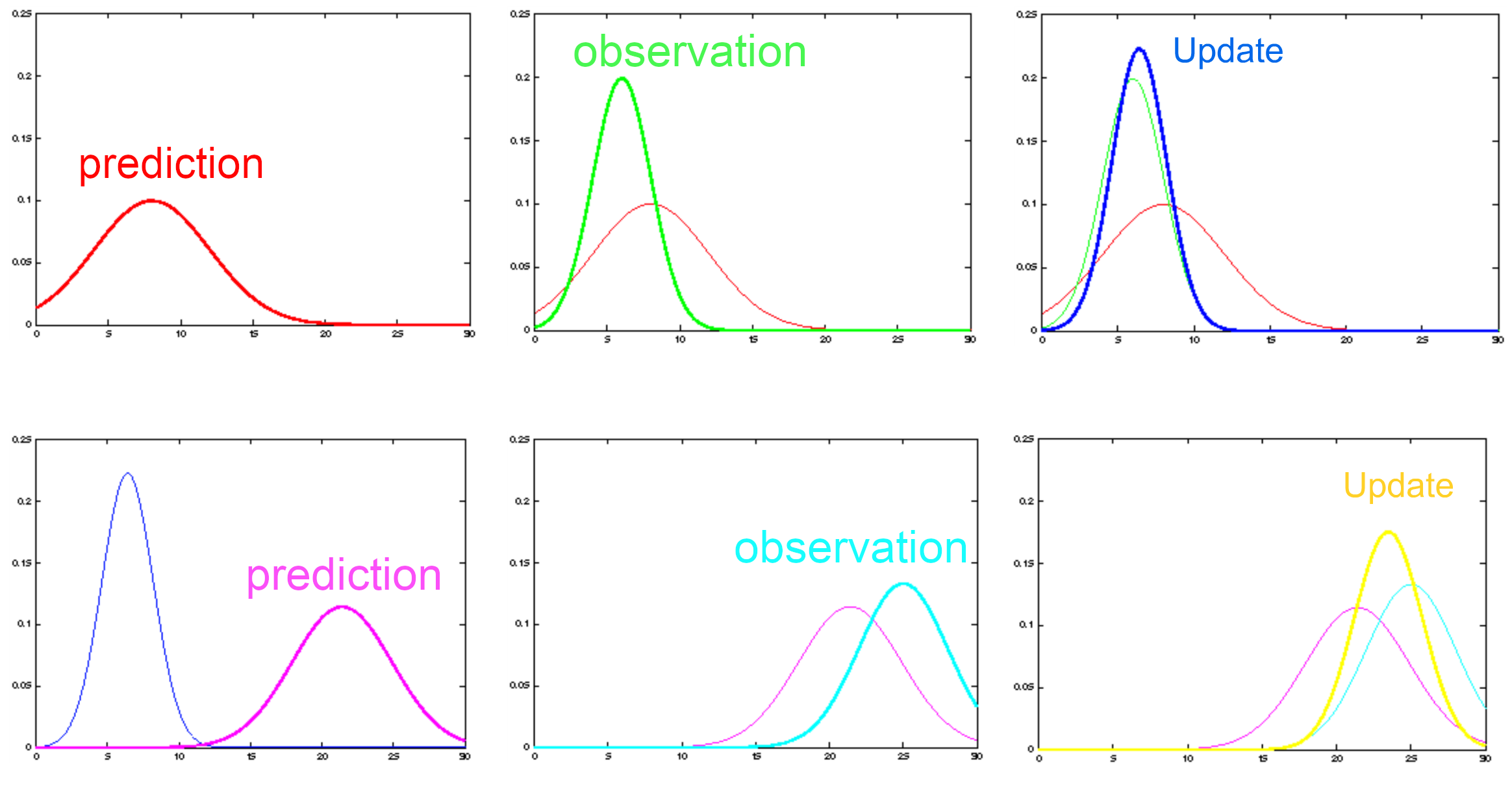
Assuming that we sequentially make predictions o

$\begin{eqnarray} \label{eq:eq-Bayes-summary01} \boldsymbol{\mu}_t^-&=\boldsymbol{\Phi}_t\boldsymbol{\mu}_{t-1}^{+}+\boldsymbol{B}_t\boldsymbol{u}_t\\ \boldsymbol{\Sigma}_t^-&=\boldsymbol{\Phi}_t\boldsymbol{\Sigma}_{t-1}^{+}\boldsymbol{\Phi}^T_t+\boldsymbol{Q}_t \end{eqnarray}$

and update the state and its covariance

$\begin{eqnarray} \label{eq:eq-Bayes-summary02} \boldsymbol{K}_t&=\boldsymbol{\Sigma}_t^{-}\boldsymbol{H}^T_t(\boldsymbol{H}_t\boldsymbol{\Sigma}_t^{-}\boldsymbol{H}^T_t+\boldsymbol{R}_t)^{-1}\\ \boldsymbol{\mu}_t^{+}&=\boldsymbol{\mu}_t^{-}+\boldsymbol{K}_t(\boldsymbol{z}_t-\boldsymbol{H}_t\boldsymbol{\mu}_t^{-}) \\ \boldsymbol{\Sigma}_t&=(\boldsymbol{I}-\boldsymbol{K}_t\boldsymbol{H}_t)\boldsymbol{\Sigma}_t^{-} \end{eqnarray}$

we can use the Kalman filter as the optimal Bayesian estimator assuming that all uncertainties are modeled by multivariate Gaussians. This is visualized in the following figure as well.

Kalman filter as Bayesing estimator based on Gaussians

Square root implementation of the Kalman filter

There are many reasons, why the covariance matrix of Kalman Filter can become singular. Mostly very small variances of the process noise or measurement noise, large differences in the magnitude of the state parameters or generally weakly conditions observation conditions, lead to singular or close-to singular matrices. In order to overcome or slightly improve such conditions, it is possible to describe the Kalman filter in its so-called square root form. Therefore it is important to understand how the square root of a matrix can be computed. Basically there are the following two possibilites for defining the square root of a matrix $\boldsymbol{A}$

$\begin{equation} \label{eq:eq-SQR01} \boldsymbol{A} = \sqrt{\boldsymbol{A}}^T \sqrt{\boldsymbol{A}} \quad \text{resp.} \quad \boldsymbol{A^2} = \boldsymbol{A}^T \boldsymbol{A} \end{equation}$

Either of the two definitions can be achieved by the following three matrix decomposition methods

Cholesky-Decomposition
$\begin{equation} \label{eq:eq-SQR02} \boldsymbol{A} = \boldsymbol{\Gamma}_{\boldsymbol{A}}^T \boldsymbol{\Gamma}_{\boldsymbol{A}} \end{equation}$
QR-Decomposition
$\begin{eqnarray} \label{eq:eq-SQR03} \boldsymbol{A} = \boldsymbol{Q} \boldsymbol{R} \\ \boldsymbol{A}^2 = \boldsymbol{R}^T \boldsymbol{Q}^T \boldsymbol{Q}\boldsymbol{R} = \boldsymbol{R}^T \boldsymbol{R} \\ \boldsymbol{R} = \boldsymbol{\Gamma}_{\boldsymbol{A}^2} \end{eqnarray}$
SVD-Decomposition
$\begin{eqnarray} \label{eq:eq-SQR04} \boldsymbol{A} = \boldsymbol{Q} \boldsymbol{\Lambda}\boldsymbol{Q}^T \\ \boldsymbol{A}^2 = \boldsymbol{Q} \boldsymbol{\Lambda}^{1/2} \boldsymbol{\Lambda}^{1/2} \boldsymbol{Q}^T \\ \sqrt{\boldsymbol{A}} = \boldsymbol{Q} \boldsymbol{\Lambda}^{1/2} \end{eqnarray}$
We (and INSTINCT) will make use of the QR decomposition in order to handle the Kalman filter in square root form. However, for the initialization of the filter, one needs to compute the square root of the initial covariance matrix. This is happening via a simple Cholesky decompositon. After that, only QR decompositions of the type
$\begin{equation} \label{eq:eq-SQR05} \boldsymbol{Q}, \boldsymbol{R} = qr\left( \begin{bmatrix} \sqrt{\boldsymbol{A}} \\ \sqrt{\boldsymbol{B}} \end{bmatrix} \right) \end{equation}$
are needed. If we define the operator $qr_R (\cdot,\cdot)$ which returns us the $\boldsymbol{R}$ matrix of the QR decomposition, we can write
$\begin{equation} \label{eq:eq-SQR06} \boldsymbol{R} = qr_R ( \sqrt{\boldsymbol{A}},\sqrt{\boldsymbol{B}}) \end{equation}$
If can be easily proven that $\boldsymbol{R}$ represents
$\begin{equation} \label{eq:eq-SQR07} \boldsymbol{R} = \sqrt{\boldsymbol{A} +\boldsymbol{B}} \end{equation}$

If we start with the prediction step

$\begin{equation} \label{eq:eq-SQR08} \boldsymbol{\Sigma}_t^- =\boldsymbol{\Phi}_t\boldsymbol{\Sigma}_{t-1}^+\boldsymbol{\Phi}^T_t+\boldsymbol{Q}_t \end{equation}$

We can write this (assuming we have Cholesky decomposed the covariance matrix and the process noise matrix) as

$\begin{equation} \label{eq:eq-SQR09} \boldsymbol{\Gamma}^T_{\boldsymbol{\Sigma}_t^-} \boldsymbol{\Gamma}_{\boldsymbol{\Sigma}_t^-} =\boldsymbol{\Phi}_t \boldsymbol{\Gamma}^T_{\boldsymbol{\Sigma}_{t-1}^+} \boldsymbol{\Gamma}_{\boldsymbol{\Sigma}_{t-1}^+} \boldsymbol{\Phi}^T_t+ \boldsymbol{\Gamma}^T_{\boldsymbol{Q}_t} \boldsymbol{\Gamma}_{\boldsymbol{Q}_t} \end{equation}$

This relation can also be written in the form

$\begin{equation} \label{eq:eq-SQR10} \boldsymbol{\Gamma}^T_{\boldsymbol{\Sigma}_t^-} \boldsymbol{\Gamma}_{\boldsymbol{\Sigma}_t^-} = \begin{bmatrix} \boldsymbol{\Phi}_t\boldsymbol{\Gamma}^T_{\boldsymbol{\Sigma}_{t-1}^+} & \boldsymbol{\Gamma}^T_{\boldsymbol{Q}_t} \end{bmatrix} \begin{bmatrix} \boldsymbol{\Gamma}_{\boldsymbol{\Sigma}_{t-1}^+}\boldsymbol{\Phi}_t^T \\ \boldsymbol{\Gamma}_{\boldsymbol{Q}_t} \end{bmatrix} \end{equation}$

Thus, as shown before, we can use the QR decomposition to obtain

$\begin{equation} \label{eq:eq-SQR11} \boldsymbol{\Gamma}_{\boldsymbol{\Sigma}_t^-} = qr_R ( \boldsymbol{\Gamma}_{\boldsymbol{\Sigma}_{t-1}^+}\boldsymbol{\Gamma}^T_{\boldsymbol{Q}_t} , \boldsymbol{\Gamma}_{\boldsymbol{Q}_t}) \end{equation}$

The update step is a little bit more complicated, as we need to compute the Kalman gain by the help of the innovation matrix. Thus, the latter is QR decomposed first

$\begin{equation} \label{eq:eq-SQR12} \boldsymbol{\Gamma}_{\boldsymbol{S}_t} = qr_R ( \boldsymbol{\Gamma}_{\boldsymbol{\Sigma}_{t}^-}\boldsymbol{H}_t^T , \boldsymbol{\Gamma}_{\boldsymbol{R}_t}) \end{equation}$

where $\boldsymbol{\Gamma}_{\boldsymbol{R}_t}$ is the square root of the measurement noise matrix (note: since this matrix is usually a diagonal matrix this square root of it can be compute straightforward without Cholesky decomposition) One can now compute the Kalman gain as

$\begin{equation} \label{eq:eq-SQR13} \boldsymbol{K}_t = \left( \boldsymbol{\Gamma}_{\boldsymbol{S}_t}^{-1} (\boldsymbol{\Gamma}_{\boldsymbol{S}_t}^{-1})^T \boldsymbol{H}_t \boldsymbol{\Gamma}^T_{\boldsymbol{\Sigma}_t^-} \boldsymbol{\Gamma}_{\boldsymbol{\Sigma}_t^-} \right)^T \end{equation}$

With that one can compute the updated (square root) covariance matrix as

$\begin{equation} \label{eq:eq-SQR14} \boldsymbol{\Gamma}_{\boldsymbol{\Sigma}_t^+} = qr_R ( \boldsymbol{\Gamma}_{\boldsymbol{\Sigma}_t^-}(\boldsymbol{I} -\boldsymbol{K}_t \boldsymbol{H}_t)^T, \boldsymbol{\Gamma}_{\boldsymbol{R}_t} \boldsymbol{K}_t^T ) \end{equation}$

Prediction and update of the state works like in the standard Kalman filter, since all necessary matrices are available anyway.

Note: While the square root form of the Kalman filter provides more numerical stability, and better balancing of the matrices, this advantage is lost at the point where the user need to back-compute the covariances matrices from their square root equivalent.